Fundamentals of machine learning part 1

Introduction

Machine learning serves as the nexus between data science and software engineering, aiming to leverage data to construct predictive models seamlessly integrated into software applications or services. Achieving this objective necessitates cooperation between data scientists, who delve into and preprocess the data for model training, and software developers, who embed the models into applications for predicting new data points, a process termed inferencing.

Throughout this module, you'll delve into fundamental concepts underpinning machine learning, distinguish between various types of machine learning models, and explore methodologies for model training and evaluation. Ultimately, you'll discover how to utilize Microsoft Azure Machine Learning for model training and deployment, sans the need for coding.

Functionality of machine learning

Given its mathematical and statistical foundations, machine learning models are commonly conceptualized in mathematical contexts. At its core, a machine learning model represents a software application encapsulating a function to compute an output value based on one or multiple input values. The process of defining this function is referred to as training. Once the function is established, it can be utilized for predicting new values through inferencing.

Let's explore the steps involved in training and inferencing.

The training data consists of past observations. In most cases, the observations include the observed attributes or features of the thing being observed, and the known value of the thing you want to train a model to predict (known as the label).

In mathematical terms, you'll often see the features referred to using the shorthand variable name x, and the label referred to as y. Usually, an observation consists of multiple feature values, so x is actually a vector (an array with multiple values), like this: [x1,x2,x3,...].

To make this clearer, let's consider the examples described previously:

1. Ice Cream Sales Scenario: The features include weather measurements like temperature, rainfall, and windspeed, while the label is the number of ice creams sold. We want to predict ice cream sales based on weather conditions.

2. 
   

3. Medical Scenario (Diabetes Risk Prediction): Here, the features consist of clinical measurements such as weight and blood glucose level, with the label indicating the likelihood of diabetes (e.g., 1 for at risk, 0 for not at risk). The goal is to predict a patient's risk of diabetes based on their clinical data.

4. 
   

5. Antarctic Research Scenario (Penguin Species Prediction): The features are physical attributes of penguins like flipper length and bill width, while the label represents the penguin's species (e.g., 0 for Adelie, 1 for Gentoo, 2 for Chinstrap). The objective is to predict the species of a penguin based on its physical characteristics.

In each case, an algorithm is applied to the data to establish a relationship between the features and the label. This relationship is generalized as a calculation that maps feature values to label values. The specific algorithm chosen depends on the predictive problem at hand, but the fundamental aim is to fit the data to a function where feature values can be used to calculate the corresponding label.

The result of the algorithm is a model that encapsulates the calculation derived by the algorithm as a function - let's call it f. In mathematical notation:

y = f(x)

After completing the training phase, the trained model transitions to the inference stage, where it functions as a software program embodying the function derived during training. This model accepts input feature values and generates a prediction of the corresponding label as output. Because the output is a prediction calculated by the model's function rather than an observed value, it's commonly denoted as ŷ (pronounced "y-hat"). This symbol distinguishes predicted values from actual observed values, emphasizing their inferred nature.

Types of machine learning

There are multiple types of machine learning, and you must apply the appropriate type depending on what you're trying to predict. A breakdown of common types of machine learning is shown in the following diagram.

Supervised machine learning

Supervised machine learning is a general term for machine learning algorithms in which the training data includes both feature values and known label values. Supervised machine learning is used to train models by determining a relationship between the features and labels in past observations, so that unknown labels can be predicted for features in future cases.

Regression

Regression is indeed a type of supervised machine learning where the goal is to predict a continuous numeric value, such as the examples you've provided:

1. Predicting the number of ice creams sold (numeric value) based on features like temperature, rainfall, and windspeed.
2. Predicting the selling price of a property (numeric value) based on various features including size, number of bedrooms, and location metrics.
3. Predicting the fuel efficiency (numeric value) of a car based on features like engine size, weight, and dimensions.

On the other hand, classification is also a type of supervised machine learning, but it deals with predicting a discrete category or class label. There are two common scenarios:

1. Binary classification: Predicting whether an observation belongs to one of two classes. For example, determining whether a patient is at risk of diabetes or not based on clinical measurements.
2. Multiclass classification: Predicting which category an observation belongs to from three or more possible classes. For instance, classifying the species of a penguin based on physical attributes into Adelie, Gentoo, or Chinstrap.

Both regression and classification are powerful techniques used in supervised machine learning, each suited for different types of predictive tasks based on the nature of the label being predicted.

Binary classification

Multiclass classification

Multiclass classification extends binary classification to predict a label that represents one of multiple possible classes. For example,

Exactly! Binary classification involves predicting whether an observation belongs to one of two mutually exclusive categories or classes. Your examples illustrate this concept perfectly:

1. Predicting whether a patient is at risk for diabetes (binary outcome: at risk or not at risk) based on clinical metrics like weight, age, and blood glucose level.
2. Predicting whether a bank customer will default on a loan (binary outcome: default or not default) based on factors such as income, credit history, and age.
3. Predicting whether a mailing list customer will respond positively to a marketing offer (binary outcome: positive response or no response) based on demographic attributes and past purchases.

In each scenario, the binary classification model aims to classify the observation into one of the two possible classes, providing a binary true/false or positive/negative prediction. This type of classification is commonly used in various fields for decision-making and risk assessment tasks

The species of a penguin (Adelie, Gentoo, or Chinstrap) based on its physical measurements.

The genre of a movie (comedy, horror, romance, adventure, or science fiction) based on its cast, director, and budget.

In most scenarios that involve a known set of multiple classes, multiclass classification is used to predict mutually exclusive labels. For example, a penguin can't be both a Gentoo and an Adelie. However, there are also some algorithms that you can use to train multilabel classification models, in which there may be more than one valid label for a single observation. For example, a movie could potentially be categorized as both science fiction and comedy.

Unsupervised machine learning

Unsupervised machine learning involves training models using data that consists only of feature values without any known labels. Unsupervised machine learning algorithms determine relationships between the features of the observations in the training data.

Clustering

Clustering, the primary form of unsupervised machine learning, operates by grouping observations into discrete clusters based on similarities in their features. For instance:

• Grouping flowers: Similar flowers can be grouped together based on attributes like size, number of leaves, and number of petals.

• Segmenting customers: Clustering can identify groups of customers with similar demographic attributes and purchasing behavior, enabling businesses to target them more effectively.

Clustering resembles multiclass classification in that it categorizes observations into distinct groups. However, the key distinction lies in the absence of pre-existing cluster labels in clustering. Unlike classification, where known class labels guide the algorithm's learning process, clustering relies solely on the similarity of features to group data points.

Clustering is often employed to define classes before training a classification model. For example:

• Customer segmentation: Businesses might use clustering to segment their customer base into groups based on purchasing behavior. These segments can then inform the creation of customer classes (e.g., high-value customers, frequent small purchasers). Subsequently, the labeled data from clustering results can be utilized to train a classification model, predicting which category a new customer belongs to based on their features.
• 
  

Regression models, a type of supervised machine learning, aim to predict numeric label values based on training data containing both features and known labels. The training process typically involves several iterations:

1. Data Splitting: The training data is randomly divided into two sets: a training dataset used to train the model and a validation dataset held back to evaluate the trained model's performance.

2. Model Fitting: An appropriate algorithm, such as linear regression for regression models, is used to fit the training data and construct the model. This involves learning the relationship between the features and labels in the training dataset.

3. Validation: The model is tested using the validation dataset by making predictions for the features. These predicted labels are compared with the actual labels in the validation dataset.

4. Evaluation: Differences between the predicted and actual label values in the validation dataset are aggregated to calculate metrics indicating the model's predictive accuracy.

The training process iterates, adjusting algorithms and parameters, until an acceptable evaluation metric is achieved. This iterative approach allows for refining the model's performance and optimizing its predictive accuracy.

For instance, let's consider a simplified regression example using the ice cream sales scenario. We aim to predict the number of ice creams sold (numeric label, y) based on a single feature value (temperature, x). We'll utilize historical data containing daily temperatures and corresponding ice cream sales records. This example demonstrates the fundamental principles of training a regression model, even though real-world scenarios often involve multiple features adding complexity to the process.

Training a regression model

We'll start by splitting the data and using a subset of it to train a model. Here's the training dataset:

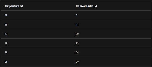
To get an insight of how these x and y values might relate to one another, we can plot them as coordinates along two axes, like this:

Now we're ready to apply an algorithm to our training data and fit it to a function that applies an operation to x to calculate y. One such algorithm is linear regression, which works by deriving a function that produces a straight line through the intersections of the x and y values while minimizing the average distance between the line and the plotted points, like this:

Exactly! In the context of linear regression, the equation of the line represents the relationship between the input feature (x) and the predicted output (y).

In our example, with the intercept at 50 on the x-axis, it means that when the temperature (our feature) is 50 degrees, the predicted ice cream sales (our label) is 0.

The slope of the line indicates the rate of change of the predicted ice cream sales with respect to changes in temperature. In this case, with a slope of 1, for every increase of 5 degrees in temperature (along the x-axis), there's a corresponding increase of 5 ice cream sales (along the y-axis).

So, the function can indeed be expressed as $�=�-50$, where $�$ is the temperature and $�$ is the predicted ice cream sales. This linear equation encapsulates the relationship between temperature and ice cream sales as learned by the linear regression model.

f(x) = x-50

You can use this function to predict the number of ice creams sold on a day with any given temperature. For example, suppose the weather forecast tells us that tomorrow it will be 77 degrees. We can apply our model to calculate 77-50 and predict that we'll sell 27 ice creams tomorrow.

But just how accurate is our model?

Evaluating a regression model

To validate the model and evaluate how well it predicts, we held back some data for which we know the label (y) value. Here's the data we held back:

We can use the model to predict the label for each of the observations in this dataset based on the feature (x) value; and then compare the predicted label (ŷ) to the known actual label value (y).

Using the model we trained earlier, which encapsulates the function f(x) = x-50, results in the following predictions:

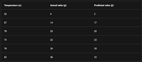
We can plot both the predicted and actual labels against the feature values like this:

The predicted labels are calculated by the model so they're on the function line, but there's some variance between the ŷ values calculated by the function and the actual y values from the validation dataset; which is indicated on the plot as a line between the ŷ and y values that shows how far off the prediction was from the actual value.

Regression evaluation metrics

Based on the differences between the predicted and actual values, you can calculate some common metrics that are used to evaluate a regression model.

Mean Absolute Error (MAE)

The variance in this example indicates by how many ice creams each prediction was wrong. It doesn't matter if the prediction was over or under the actual value (so for example, -3 and +3 both indicate a variance of 3). This metric is known as the absolute error for each prediction, and can be summarized for the whole validation set as the mean absolute error (MAE).

In the ice cream example, the mean (average) of the absolute errors (2, 3, 3, 1, 2, and 3) is 2.33.

Mean Squared Error (MSE)

The mean absolute error metric takes all discrepancies between predicted and actual labels into account equally. However, it may be more desirable to have a model that is consistently wrong by a small amount than one that makes fewer, but larger errors. One way to produce a metric that "amplifies" larger errors by squaring the individual errors and calculating the mean of the squared values. This metric is known as the mean squared error (MSE).

In our ice cream example, the mean of the squared absolute values (which are 4, 9, 9, 1, 4, and 9) is 6.

Root Mean Squared Error (RMSE)

The mean squared error helps take the magnitude of errors into account, but because it squares the error values, the resulting metric no longer represents the quantity measured by the label. In other words, we can say that the MSE of our model is 6, but that doesn't measure its accuracy in terms of the number of ice creams that were mispredicted; 6 is just a numeric score that indicates the level of error in the validation predictions.

If we want to measure the error in terms of the number of ice creams, we need to calculate the square root of the MSE; which produces a metric called, unsurprisingly, Root Mean Squared Error. In this case √6, which is 2.45 (ice creams).

Coefficient of determination (R2)

All of the metrics so far compare the discrepancy between the predicted and actual values in order to evaluate the model. However, in reality, there's some natural random variance in the daily sales of ice cream that the model takes into account. In a linear regression model, the training algorithm fits a straight line that minimizes the mean variance between the function and the known label values. The coefficient of determination (more commonly referred to as R2 or R-Squared) is a metric that measures the proportion of variance in the validation results that can be explained by the model, as opposed to some anomalous aspect of the validation data (for example, a day with a highly unusual number of ice creams sales because of a local festival).

The calculation for R2 is more complex than for the previous metrics. It compares the sum of squared differences between predicted and actual labels with the sum of squared differences between the actual label values and the mean of actual label values, like this:

R2 = 1- ∑(y-ŷ)2 ÷ ∑(y-ȳ)2

Don't worry too much if that looks complicated; most machine learning tools can calculate the metric for you. The important point is that the result is a value between 0 and 1 that describes the proportion of variance explained by the model. In simple terms, the closer to 1 this value is, the better the model is fitting the validation data. In the case of the ice cream regression model, the R2 calculated from the validation data is 0.95.

REFERENCE :- https://learn.microsoft.com/en-us/training/modules/fundamentals-machine-  learning

                       ;- open AI